PPforest
N. da Silva, D. Cook & E.K Lee
2025-07-23
Source:vignettes/PPforest-vignette.Rmd
PPforest-vignette.RmdIntroduction
The PPforest package (projection pursuit random forest)
contains functions to fit a projection pursuit random forest for
classification problems described in (da Silva,
Cook, and Lee 2021). This method utilize combinations of
variables in each tree construction. In a random forest each split is
based on a single variable, chosen from a subset of predictors. In the
PPforest, each split is based on a linear combination of
randomly chosen variables. The linear combination is computed by
optimizing a projection pursuit index, to get a projection of the
variables that best separates the classes. The PPforest
uses the PPtree algorithm (Y. D. Lee
et al. 2013), which fits a single tree to the data. Utilizing
linear combinations of variables to separate classes takes the
correlation between variables into account, and can outperform the basic
forest when separations between groups occurs on combinations of
variables. Two projection pursuit indexes, LDA and PDA, are used for
PPforest.
To improve the speed performance PPforest package,
PPtree algorithm was translated to Rcpp.
PPforest package utilizes a number of R packages some of
them included in “suggests” not to load them all at package
start-up.
You can install the package from CRAN:
Or the development version of PPforest can be installed
from github using:
library(devtools)
install_github("natydasilva/PPforest")
library(PPforest)
Projection pursuit classification forest
In PPforest, projection pursuit classification trees are
used as the individual model to be combined in the forest. The original
algorithm is in PPtreeViz package, we translate the
original tree algorithm into Rcpp to improve the speed
performance to run the forest.
One important characteristic of PPtree is that treats the data always as a two-class system, when the classes are more than two the algorithm uses a two step projection pursuits optimization in every node split. Let the data set, is a p-dimensional vector of explanatory variables and represents class information with .
In the first step optimize a projection pursuit index to find an optimal one-dimension projection for separating all classes in the current data. With the projected data redefine the problem in a two class problem by comparing means, and assign a new label or to each observation, a new variable is created. The new groups and can contain more than one original classes. Next step is to find an optimal one-dimensional projection , using to separate the two class problem and . The best separation of and is determine in this step and the decision rule is defined for the current node, if then assign to the left node else assign to the right node, where is the mean of . For each groups we can repeat all the previous steps until and have only one class from the original classes. Base on this process to grow the tree, the depth of PPtree is at most the number of classes because one class is assigned only to one final node.
Trees from PPtree algorithm are simple, they use the
association between variables to find separation. If a linear boundary
exists, PPtree produces a tree without
misclassification.
Projection pursuit random forest algorithm description
Let N the number of cases in the training set , bootstrap samples from the training set are taking (samples of size N with replacement).
For each bootstrap sample a \verb PPtree is grown to the largest extent possible . No pruning. This tree is grown using step 3 modification.
Let M the number of input variables, a number of variables are selected at random at each node and the best split based on a linear combination of these randomly chosen variables. The linear combination is computed by optimizing a projection pursuit index, to get a projection of the variables that best separates the classes.
Predict the classes of each case not included in the bootstrap sample and compute oob error.
Based on majority vote predict the class for new data.
Overview PPforest package
PPforest package implements a classification random
forest using projection pursuit classification trees. The following
table present all the functions in PPforest package.
| Function | Description |
|---|---|
| node_data | Data structure with the projected and boundary by node and class |
| permute_importance | Obtain the permuted importance variable measure |
| ppf_avg_imp | Computes a global importance measure for a PPforest object, average importance measure for a pptree over all the trees. |
| ppf_global_imp | Computes a global importance measure for a PPforest object |
| PPforest | Runs a Projection pursuit random forest |
| PPtree_split | Projection pursuit classification tree with random variable selection in each split |
| print.PPforest | Print PPforest object |
| predict.PPforest | Predict class for the test set and calculate prediction error |
| ternary_str | Data structure with the projected and boundary by node and class |
Also PPforest package includes some data set that were
used to test the predictive performance of our method. The data sets
included are: crab, fishcatch, glass, image, leukemia, lymphoma NCI60,
parkinson and wine.
Example
Australian crab data set will be used as example. This data contains measurements on rock crabs of the genus Leptograpsus. There are 200 observations from two species (blue and orange) and for each specie (50 in each one) there are 50 males and 50 females. Class variable has 4 classes with the combinations of specie and sex (BlueMale, BlueFemale, OrangeMale and OrangeFemale). The data were collected on site at Fremantle, Western Australia. For each specimen, five measurements were made, using vernier calipers.
- FL the size of the frontal lobe length, in mm
- RW rear width, in mm
- CL length of mid line of the carapace, in mm
- CW maximum width of carapace, in mm
- BD depth of the body; for females, measured after displacement of the abdomen, in mm
To visualize this data set we use a scatterplot matrix from the
package GGally
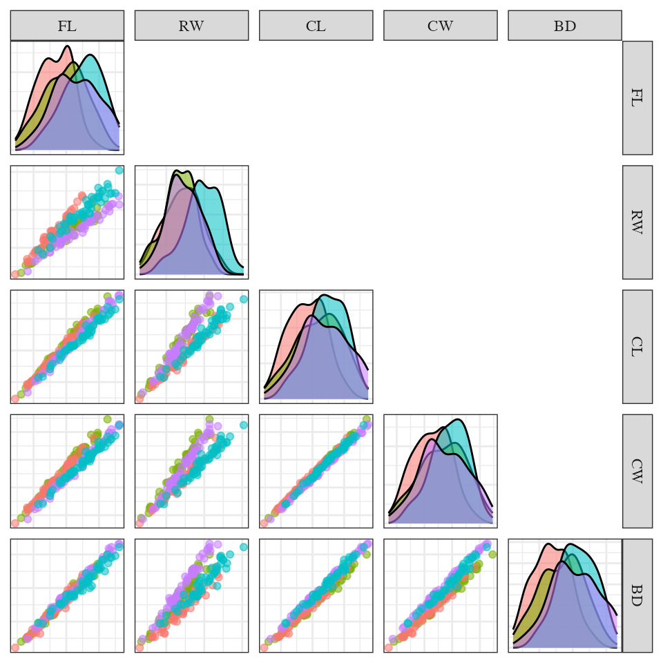
Scatter plot matrix of crab data
In this figure we can see a strong, positive and linear association between the different variables. Also look like the classes can be separated by linear combinations.
The main function of the package is PPforest which
implements a projection pursuit random forest.
PPtree_split this function implements a projection
pursuit classification tree with random variable selection in each
split, based on the original PPtree algorithm from
PPtreeViz R package (E.-K. Lee
2018). This function returns a PPtreeclass object.
To use this function we need to specify a formula describing the model
to be fitted response~predictors (form), data
is a data frame with the complete data set. Also we need to specify the
method PPmethod, it is the index to use for projection
pursuit: ‘LDA’ or ‘PDA’, size.p is the proportion of
variables randomly sampled in each split. If size.p = 1 a classic
PPtreeclass object will be fitted using all the variables
in each node partition instead of a subset of them. lambda
penalty parameter in PDA index and is between 0 to 1 . he following
example fits a projection pursuit classification tree constructed using
0.6 of the variables (3 out of 5) in each node split. We selected
LDA method.
Tree.crab <- PPforest::PPtree_split("Type~.", data = crab, PPmethod = "LDA", size.p = 0.6)
 Tree.crab
## =============================================================
## Projection Pursuit Classification Tree result
## =============================================================
##
## 1) root
## 2) proj1*X < cut1
## 4)* proj2*X < cut2 -> "BlueMale"
## 5)* proj2*X >= cut2 -> "BlueFemale"
## 3) proj1*X >= cut1
## 6)* proj3*X < cut3 -> "OrangeMale"
## 7)* proj3*X >= cut3 -> "OrangeFemale"
##
## Error rates of various cutoff values
## -------------------------------------------------------------
## Rule1 Rule2 Rule3 Rule4 Rule5 Rule6 Rule7 Rule8
## error.rate 0.065 0.065 0.065 0.065 0.075 0.075 0.075 0.075PPforest function runs a projection pursuit random
forest. The arguments are data a data.frame with the data
information, y a character with the name of the class
variable. size.tr to specify the proportion of observations
using in the training. Using this function we have the option to split
the data in training and test using size.tr internally in
the PPforest function. size.tr is the
proportion of data used in the training and the test proportion will be
1- size.tr. The number of trees in the forest is specified
using the argument m. The argument size.p is
the sample proportion of the variables used in each node split,
PPmethod is the projection pursuit index to be optimized,
two options LDA and PDA are available. The algorithm can be parallelized
using parallel and cores arguments.
pprf.crab <- PPforest::PPforest(data = crab, y = "Type", std = 'min-max', size.tr = .7, m = 200,
                                size.p =  .8,  PPmethod = 'LDA',  parallel = TRUE, cores = 2)

pprf.crab
##
## Call:
## PPforest::PPforest(data = crab, y = "Type", std = "min-max", size.tr = 0.7, m = 200, PPmethod = "LDA", size.p = 0.8, parallel = TRUE, cores = 2)
## Type of random forest: Classification
## Number of trees: 200
## No. of variables tried at each split: 4
##
## OOB estimate of error rate: 5.71%
## Confusion matrix:
## BlueFemale BlueMale OrangeFemale OrangeMale class.error
## BlueFemale 33 2 0 0 0.06
## BlueMale 4 31 0 0 0.11
## OrangeFemale 0 0 33 2 0.06
## OrangeMale 0 0 0 35 0.00PPforest print a summary result from the model with the
confusion matrix information and the oob-error rate in a similar way
randomForest packages does.
This function returns the predicted values of the training data, training error, test error and predicted test values. Also there is the information about out of bag error for the forest and also for each tree in the forest. Bootstrap samples, output of all the trees in the forest from , proximity matrix and vote matrix, number of trees grown in the forest, number of predictor variables selected to use for splitting at each node. Confusion matrix of the prediction (based on OOb data), the training data and test data and vote matrix are also returned.
The printed version of a PPforest object follows the
randomForest printed version to make them comparable. Based
on confusion matrix, we can observe that the biggest error is for
BlueMale class. Most of the wrong classified values are between
BlueFemale and BlueMale.
The output from a PPforest object contains a lot of
information as we can see in the next output.
str(pprf.crab, max.level = 1 )## List of 28
## $ predicting.training: Factor w/ 4 levels "BlueFemale","BlueMale",..: 2 2 2 1 2 2 2 1 2 2 ...
## $ training.error : num 0.05
## $ prediction.test : Factor w/ 4 levels "BlueFemale","BlueMale",..: 2 2 2 1 2 1 2 2 2 2 ...
## $ error.test : num 0.0833
## $ oob.error.forest : num 0.0571
## $ oob.error.tree : num [1:200, 1] 0.1346 0.06 0.08 0.08 0.0222 ...
## $ boot.samp :List of 200
## $ output.trees :List of 200
## $ proximity : num [1:140, 1:140] 0 0.805 0.825 0.35 0.835 0.675 0.665 0.625 0.805 0.635 ...
## $ votes : num [1:140, 1:4] 0.342 0.514 0.2 0.701 0.175 ...
## ..- attr(*, "dimnames")=List of 2
## $ prediction.oob : Factor w/ 4 levels "BlueFemale","BlueMale",..: 2 1 2 1 2 2 2 1 2 2 ...
## $ n.tree : num 200
## $ n.var : int 4
## $ type : chr "Classification"
## $ confusion : num [1:4, 1:5] 33 4 0 0 2 31 0 0 0 0 ...
## ..- attr(*, "dimnames")=List of 2
## $ call : language PPforest::PPforest(data = crab, y = "Type", std = "min-max", size.tr = 0.7, m = 200, PPmethod = "LDA", size.| __truncated__
## $ train :'data.frame': 140 obs. of 6 variables:
## $ test :'data.frame': 60 obs. of 6 variables:
## $ vote.mat : num [1:200, 1:140] 2 4 2 2 2 2 2 2 2 1 ...
## ..- attr(*, "dimnames")=List of 2
## $ vote.mat_cl : chr [1:4] "BlueFemale" "BlueMale" "OrangeFemale" "OrangeMale"
## $ class.var : chr "Type"
## $ oob.obs : num [1:200, 1:140] 0 0 0 1 0 1 0 0 0 0 ...
## $ std : chr "min-max"
## $ dataux : tibble [140 × 5] (S3: tbl_df/tbl/data.frame)
## $ mincol : Named num [1:5] 8.1 6.7 16.1 18.6 7
## ..- attr(*, "names")= chr [1:5] "FL" "RW" "CL" "CW" ...
## $ maxmincol : Named num [1:5] 15 13.5 31.5 36 14.6
## ..- attr(*, "names")= chr [1:5] "FL" "RW" "CL" "CW" ...
## $ train_mean : NULL
## $ train_sd : NULL
## - attr(*, "class")= chr "PPforest"For example to get the predicted values for the test data we can use the PPforest output:
pprf.crab$prediction.test## [1] BlueMale BlueMale BlueMale BlueFemale BlueMale
## [6] BlueFemale BlueMale BlueMale BlueMale BlueMale
## [11] BlueMale BlueMale BlueMale BlueMale BlueMale
## [16] BlueMale BlueFemale BlueFemale BlueFemale BlueFemale
## [21] BlueFemale BlueFemale BlueFemale BlueFemale BlueFemale
## [26] BlueFemale BlueFemale BlueFemale BlueFemale BlueFemale
## [31] OrangeMale OrangeMale OrangeMale OrangeMale OrangeMale
## [36] OrangeMale OrangeMale OrangeMale OrangeMale OrangeMale
## [41] OrangeMale OrangeMale OrangeMale OrangeMale OrangeMale
## [46] OrangeMale OrangeMale OrangeFemale OrangeFemale OrangeFemale
## [51] OrangeFemale OrangeFemale OrangeFemale OrangeFemale OrangeFemale
## [56] OrangeFemale OrangeFemale OrangeFemale OrangeFemale OrangeFemale
## Levels: BlueFemale BlueMale OrangeFemale OrangeMaleIf new data are available you can use the function
trees_pred to get the predicted classes by PPforest
object.
predict(object = pprf.crab, newdata)
The PPforest algorithm calculates variable importance in two ways: (1) permuted importance using accuracy, and (2) importance based on projection coefficients on standardized variables.
The permuted variable importance is comparable with the measure defined in the classical random forest algorithm. It is computed using the out of bag (oob) sample for the tree for each predictor variable. Then the permuted importance of the variable in the tree can be defined as:
where is the predicted class for the observation in the tree and is the predicted class for the observation in the tree after permuting the values for variable . The global permuted importance measure is the average importance over all the trees in the forest. This measure is based on comparing the accuracy of classifying out-of-bag observations, using the true class with permuted (nonsense) class. To compute this measure you should use permute_importance function.
impo1 <- permute_importance(pprf.crab)
impo1
## nm imp sd.imp imp2 sd.imp2 imp2.std imp.std
## 1 BD 17.285 7.678448 0.3403903 0.1465104 2.323318 2.251106
## 2 RW 18.295 6.377408 0.3615318 0.1231153 2.936530 2.868720
## 3 CW 21.465 6.615710 0.4245943 0.1291092 3.288646 3.244550
## 4 CL 21.790 7.267737 0.4300271 0.1394407 3.083942 2.998182
## 5 FL 22.215 7.564714 0.4397407 0.1462055 3.007689 2.936661
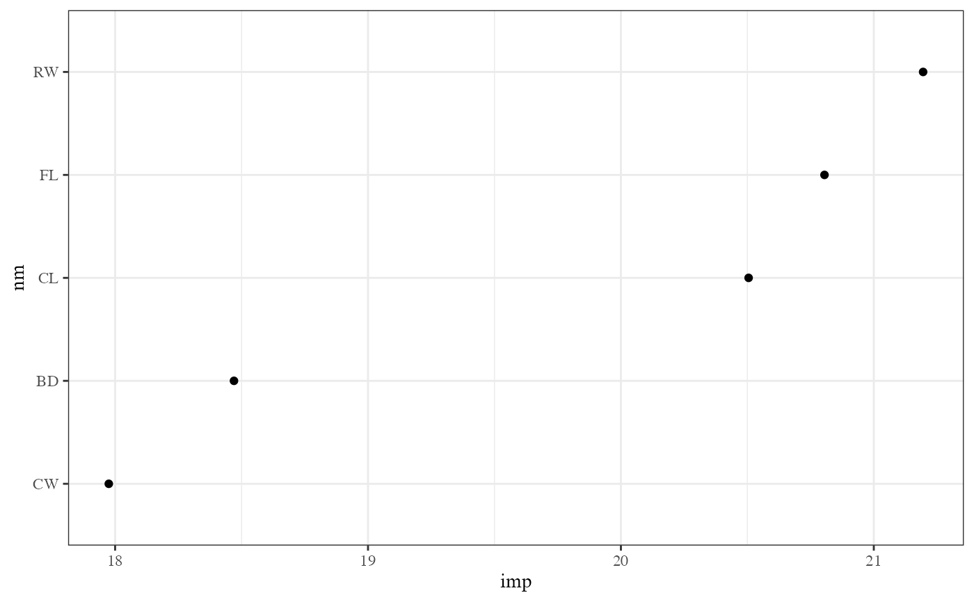
Permuted importance variable
This function returns a data frame with permuted importance measures, imp is the permuted importance measure defined in Brieman paper, imp2 is the permuted importance measure defined in randomForest package, the standard deviation (sd.im and sd.imp2) for each measure is computed and the also the standardized measure.
For the second importance measure, the coefficients of each projection are examined. The magnitude of these values indicates importance, if the variables have been standardized. The variable importance for a single tree is computed by a weighted sum of the absolute values of the coefficients across nodes. The weights takes the number of classes in each node into account (Y. D. Lee et al. 2013). Then the importance of the variable in the PPtree can be defined as:
Where is the projected coefficient for node and variable and the total number of node partitions in the tree .
The global variable importance in a PPforest then can be defined in different ways. The most intuitive is the average variable importance from each PPtree across all the trees in the forest.
Alternatively we have defined a global importance measure for the forest as a weighted mean of the absolute value of the projection coefficients across all nodes in every tree. The weights are based on the projection pursuit indexes in each node (), and 1-(OOB-error of each tree)().
impo2 <-  ppf_avg_imp(pprf.crab, "Type")
impo2
## # A tibble: 5 × 2
## variable mean
## <fct> <dbl>
## 1 CL 0.573
## 2 CW 0.532
## 3 RW 0.431
## 4 FL 0.294
## 5 BD 0.185
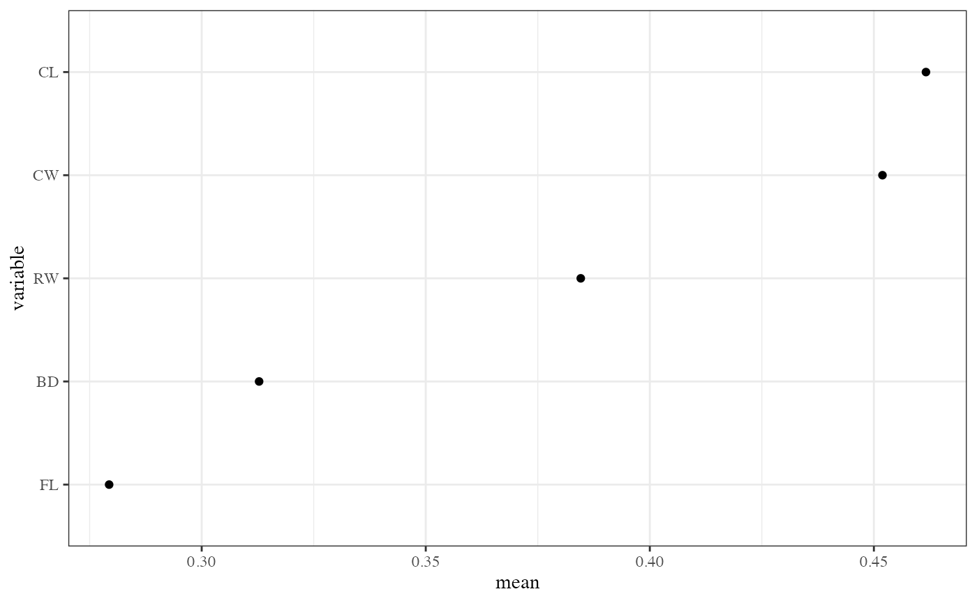
Average importance variable
Finally you can get the last importance measure we have proposed for the PPforest using `ppf_global_imp’ function.
impo3 <- ppf_global_imp(data = crab, y = "Type", pprf.crab)
impo3
## # A tibble: 5 × 2
## variable mean
## <fct> <dbl>
## 1 CW 0.421
## 2 CL 0.381
## 3 RW 0.273
## 4 FL 0.225
## 5 BD 0.150
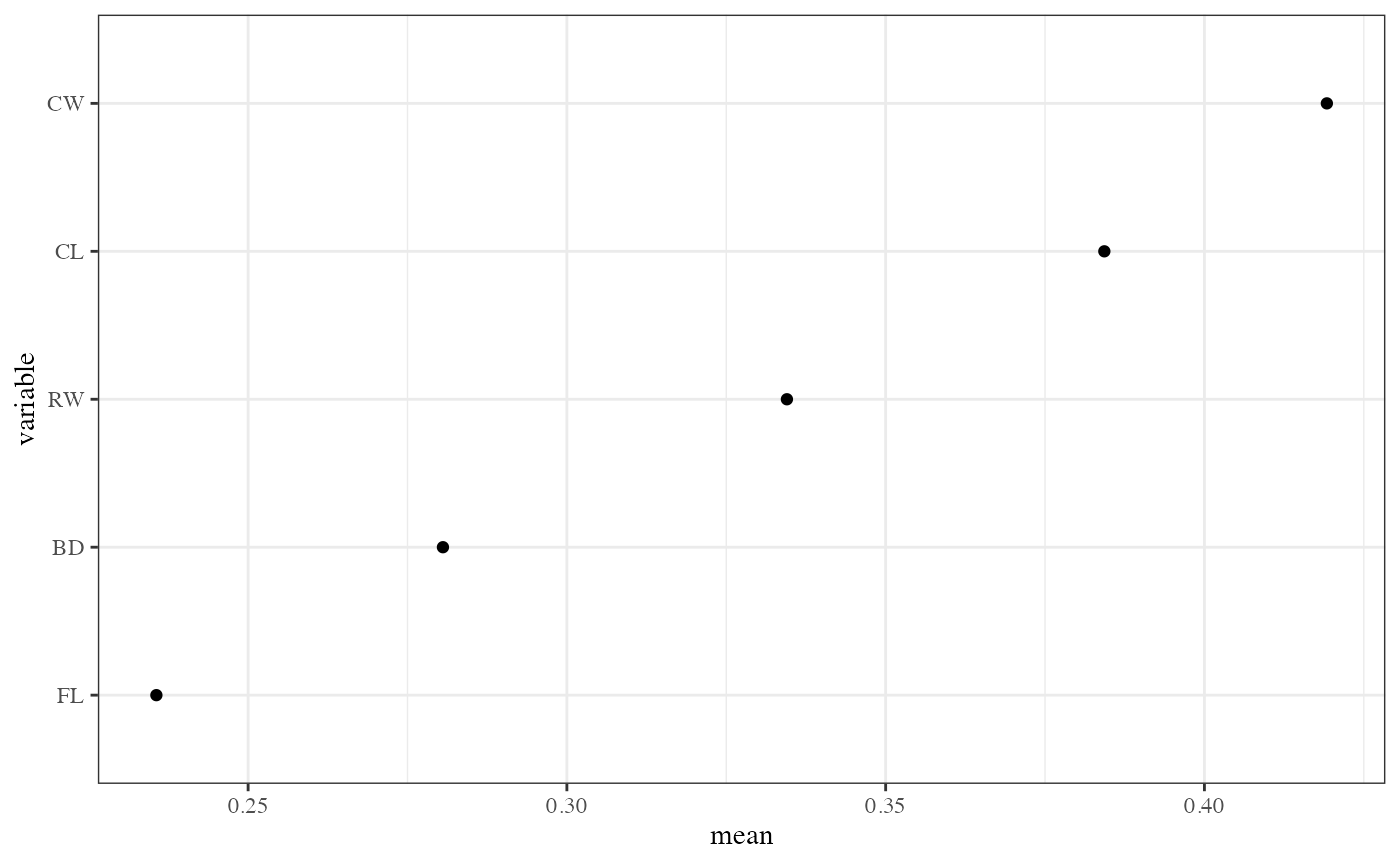
Global importance variable
Using the information available in the PPforest object, some visualization can be done. I will include some useful examples to visualize the data and some of the most important diagnostics in a forest structure.
To describe the data structure a parallel plot can be done, the data were standardized and the color represents the class variable.
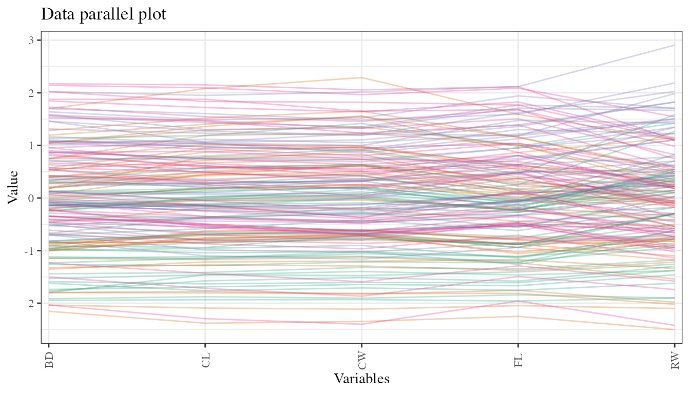
Parallel coordinate plot of crab data
ternary_str is an auxiliary functions in
PPforest to get the data structure needed to do a ternary
plot or a generalized ternary plot if more than 3 classes are available.
Because the PPforest is composed of many tree fits on subsets of the
data, a lot of statistics can be calculated to analyze as a separate
data set, and better understand how the model is working. Some of the
diagnostics of interest are: variable importance, OOB error rate, vote
matrix and proximity matrix.
With a decision tree we can compute for every pair of observations the proximity matrix. This is a matrix where if two cases and are in the same terminal node increase their proximity by one, at the end normalize the proximities by dividing by the number of trees. To visualize the proximity matrix we use a scatter plot with information from multidimensional scaling method. In this plot color indicates the true species and sex. For this data two dimensions are enough to see the four groups separated quite well. Some crabs are clearly more similar to a different group, though, especially in examining the sex differences.
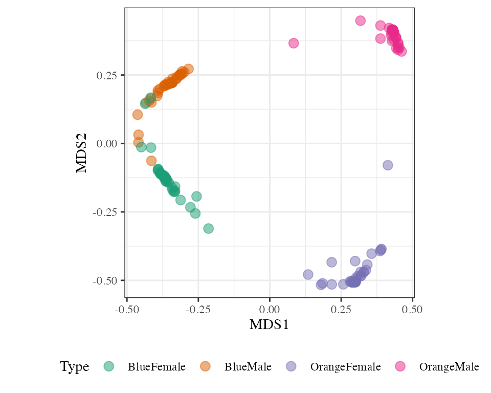
Multidimensional scaling plot to examine similarities between cases
The vote matrix () contains the proportion of times each observation was classified to each class, whole oob. Two possible approaches to visualize the vote matrix information are shown, with a side-by-side jittered dot plot or with ternary plots. A side-by-side jittered dotplot is used for the display, where class is displayed on one axis and proportion is displayed on the other. For each dotplot, the ideal arrangement is that points of observations in that class have values bigger than 0.5, and all other observations have less. This data is close to the ideal but not perfect, e.g. there are a few blue male crabs (orange) that are frequently predicted to be blue females (green), and a few blue female crabs predicted to be another class.
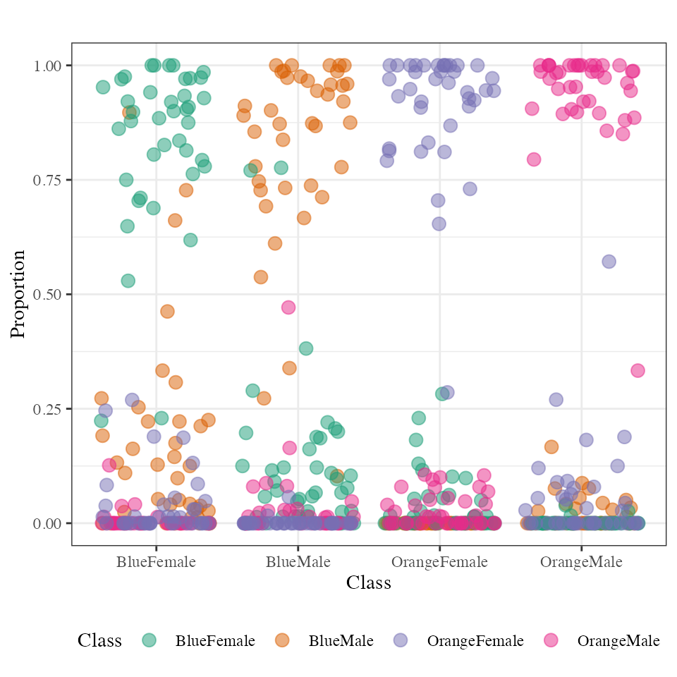
Vote matrix representation by a jittered side-by-side dotplot. Each dotplot shows the proportion of times the case was predicted into the group, with 1 indicating that the case was always predicted to the group and 0 being never.
A ternary plot is a triangular diagram that shows the proportion of three variables that sum to a constant and is done using barycentric coordinates. Compositional data lies in a -D simplex in -space. One advantage of ternary plot is that are good to visualize compositional data and the proportion of three variables in a two dimensional space can be shown. When we have tree classes a ternary plot are well defined. With more than tree classes the ternary plot idea need to be generalized.@sutherland2000orca suggest the best approach to visualize compositional data will be to project the data into the D space (ternary diagram in ) This will be the approach used to visualize the vote matrix information.
A ternary plot is a triangular diagram used to display compositional data with three components. More generally, compositional data can have any number of components, say , and hence is contrained to a -D simplex in -space. The vote matrix is an example of compositional data, with components.
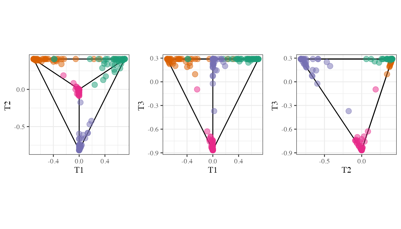
Generalized ternary plot representation of the vote matrix for four classes. The tetrahedron is shown pairwise. Each point corresponds to one observation and color is the true class.
To see a complete description about how to visualize a PPforest object read Interactive Graphics for Visually Diagnosing Forest Classifiers in R (da Silva, Cook, and Lee 2025).