High-Dimensional Classification Boundaries • classbound

The problem with more than two features

A boundary plot requires two axes. When a classifier is trained on more than two features, there is no single 2D picture that faithfully represents the full decision boundary. The boundary exists in a higher-dimensional space.

classbound provides two strategies for visualizing high-dimensional boundaries:

Strategy	What it shows
2D Slice	Two selected features on the axes; all other features are fixed at reference values
Projection	All features combined into two projected axes via a linear transformation

Neither is universally better. Which to choose depends on your question.

Setup

library(classbound)
library(palmerpenguins)

# Use three numeric features from palmerpenguins
penguins <- na.omit(palmerpenguins::penguins[
  ,
  c("species", "bill_length_mm", "bill_depth_mm", "flipper_length_mm")
])

# Fit a decision tree on all three features
m3 <- fit_model(
  penguins, species ~ bill_length_mm + bill_depth_mm + flipper_length_mm,
  rpart::rpart
)
m3
#> === Classbound Model Pipeline ===
#> Features:  bill_length_mm, bill_depth_mm, flipper_length_mm 
#> Classes:   Adelie, Chinstrap, Gentoo 
#> Boundary: Not yet computed (Run `boundary_compute()`)
#> 
#> -- Native Model --
#> n= 342 \n\nnode), split, n, loss, yval, (yprob)\n      * denotes terminal node\n\n1) root 342 191 Adelie (0.441520468 0.198830409 0.359649123)  \n  2) flipper_length_mm< 206.5 213  64 Adelie (0.699530516 0.295774648 0.004694836)  \n    4) bill_length_mm< 43.35 150   5 Adelie (0.966666667 0.033333333 0.000000000) *\n    5) bill_length_mm>=43.35 63   5 Chinstrap (0.063492063 0.920634921 0.015873016) *\n  3) flipper_length_mm>=206.5 129   7 Gentoo (0.015503876 0.038759690 0.945736434)  \n    6) bill_depth_mm>=17.65 7   2 Chinstrap (0.285714286 0.714285714 0.000000000) *\n    7) bill_depth_mm< 17.65 122   0 Gentoo (0.000000000 0.000000000 1.000000000) *

2D Slice

A 2D slice selects two features as the plot axes and holds all other features fixed at their training-set median (for numeric features) or mode (for categorical features).

The slice shows how the classifier behaves at a particular cross-section of the feature space. Two observations that appear in the same region may be separated by the classifier in a dimension that is being held fixed.

# Visualize bill_length_mm vs bill_depth_mm
# flipper_length_mm is automatically fixed at its training-set median
m3_slice <- boundary_compute(
  m3,
  feature_range = list(bill_length_mm = c(30, 60), bill_depth_mm = c(10, 25)),
  resolution    = 60
)

plot_boundary(
  m3_slice,
  obs_data   = penguins,
  x_col      = "bill_length_mm",
  y_col      = "bill_depth_mm",
  true_label = "species"
)

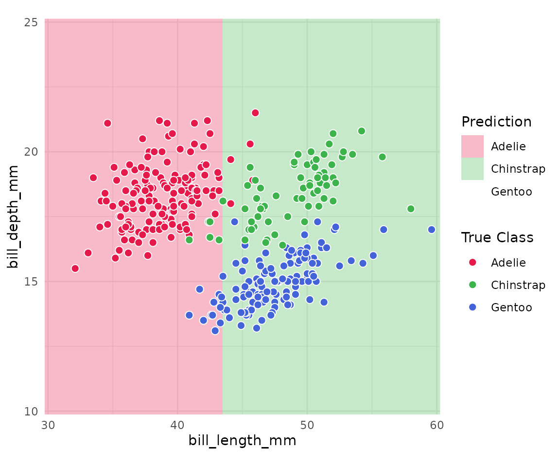
The warning message tells you which features were automatically imputed, and at what values. You can override this with the reference argument:

# Fix flipper_length_mm at a specific value instead of the median
m3_slice2 <- boundary_compute(
  m3,
  feature_range = list(bill_length_mm = c(30, 60), bill_depth_mm = c(10, 25)),
  resolution    = 60,
  reference     = list(flipper_length_mm = 200)
)

plot_boundary(m3_slice2,
  obs_data = penguins,
  x_col = "bill_length_mm", y_col = "bill_depth_mm",
  true_label = "species"
)

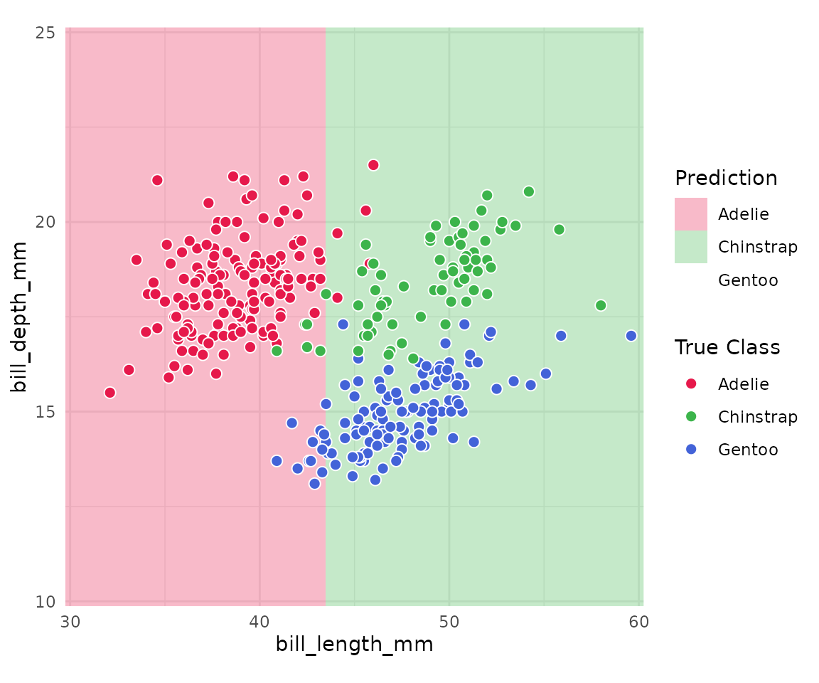
The boundary shape changes as the reference value changes, because a different slice through the 3D boundary is being rendered.

Projection

A projection collapses all features into two new axes by multiplying the feature matrix by a 2-column basis matrix. Rather than holding features fixed, it combines them: each projected point summarizes information from all original features simultaneously.

Note on Explorapp vs Scripts: In the explorapp() interactive UI, Projection mode uses PCA automatically. In the programmatic API (like the script below), you provide the projection matrix yourself, allowing you to use PCA, tourr projections, or any other projection method of your choice.

The basis must be an orthonormal matrix (columns are unit vectors, perpendicular to each other). PCA rotation matrices satisfy this by construction.

feat_cols <- c("bill_length_mm", "bill_depth_mm", "flipper_length_mm")

# Compute PCA on the three numeric features
pca <- prcomp(penguins[, feat_cols], scale. = TRUE)
basis <- pca$rotation[, 1:2] # first two principal components

# Project the training data manually to get axis ranges
x_mat <- scale(penguins[, feat_cols], center = pca$center, scale = pca$scale)
z_mat <- x_mat %*% basis

# Compute boundary in projected space, inverse-project for prediction
m3_proj <- boundary_compute(
  m3,
  feature_range = list(
    PC1 = range(z_mat[, 1]) + c(-0.5, 0.5),
    PC2 = range(z_mat[, 2]) + c(-0.5, 0.5)
  ),
  resolution = 60,
  projection = list(basis = basis, center = pca$center, scale = pca$scale)
)

plot_boundary(
  m3_proj,
  obs_data   = penguins,
  x_col      = "PC1",
  y_col      = "PC2",
  true_label = "species"
)

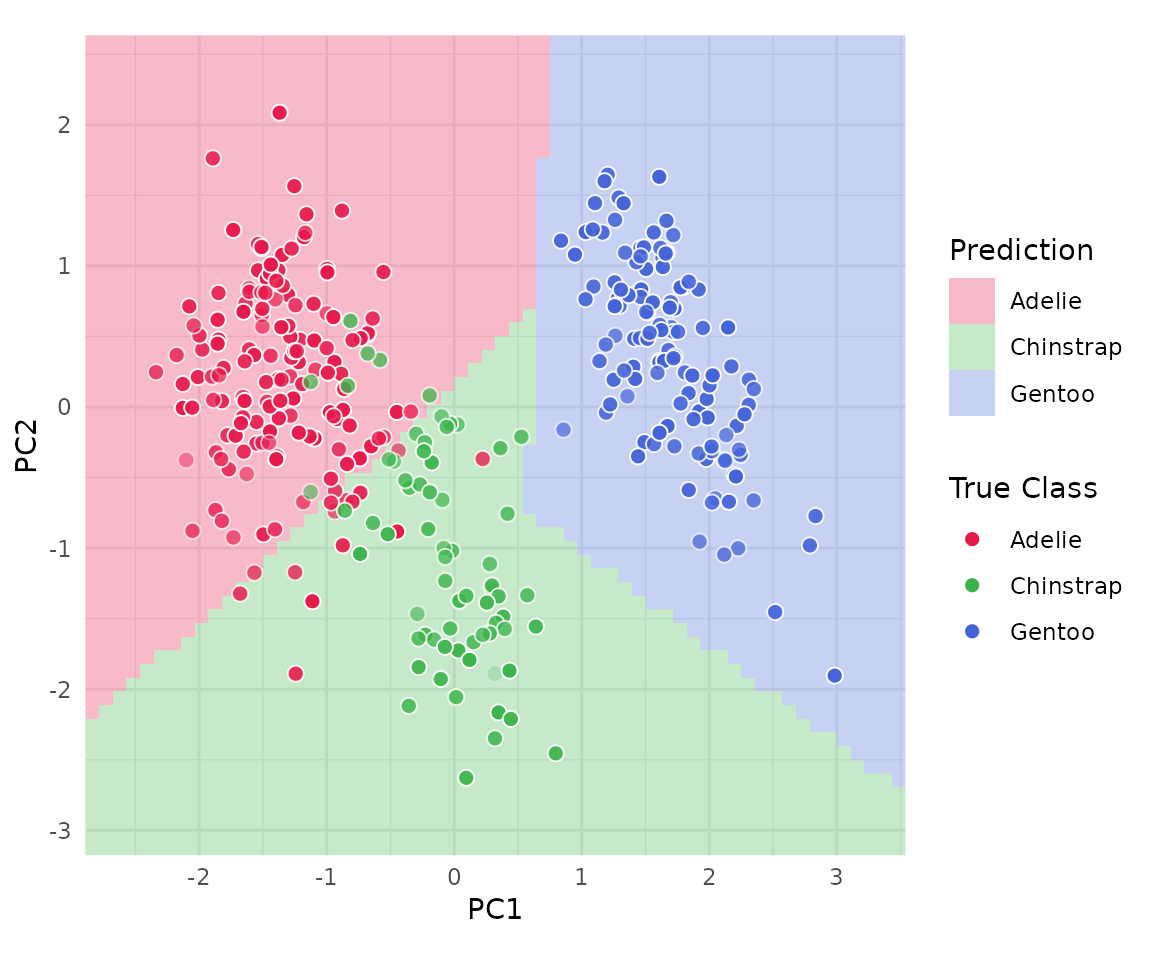
Points are forward-projected onto the plane for overlay. Points that are far from the projection plane in the original 3D space are rendered with lower opacity (depth fading), giving a visual indication of how faithfully each point’s position is captured.

When to use each strategy

2D Slice is the right choice when: - You want to examine how a specific pair of features interacts - Other dimensions are genuinely unimportant or you want to hold them constant - You want to compare the boundary at different values of a third variable

Projection is the right choice when: - All features contribute to the boundary - You want a global overview of the multi-dimensional structure - You are using tourr to animate through different projection angles

High-dimensional data: data69_1

The package includes the UCI Waveform dataset (data69_1) with 21 numeric features and 3 classes. This dataset is better suited than palmerpenguins when genuinely high-dimensional boundary exploration is the goal.

data(data69_1)
dim(data69_1) # 5000 x 22

# Fit on first 5 features for a manageable example
d <- data69_1[1:500, c("Y", "V1", "V2", "V3", "V4", "V5")]
d$Y <- as.factor(d$Y)
m_nd <- fit_model(d, Y ~ ., rpart::rpart)

# 2D slice: V1 vs V2, others at median
m_nd_slice <- boundary_compute(m_nd,
  feature_range = list(V1 = c(-3, 3), V2 = c(-3, 3)),
  resolution    = 50
)

plot_boundary(m_nd_slice,
  obs_data = d,
  x_col = "V1", y_col = "V2", true_label = "Y"
)

For the full high-dimensional tourr workflow using data69_1, see vignette("tourr-workflow").