Comparing Models with tourr

Overview

The tourr package generates animated sequences of linear projections (called a grand tour) that collectively show the structure of high-dimensional data from many angles. When combined with classbound, you can visualize how decision boundaries of different classifiers appear across multiple projection angles.

The key principle is to generate one shared projection sequence and apply it to all models. This ensures that when you compare boundaries side by side, each model is viewed through the exact same projection at the exact same frame.

# Install tourr if needed
install.packages("tourr")

Workflow overview

1. Prepare data (numeric features only)
2. Fit models
3. Generate one tour path via tourr::save_history()
4. For each tour frame (projection basis):
   a. Compute boundary via boundary_compute(..., projection = list(basis = frame))
   b. Forward-project observations for overlay
   c. Plot with plot_boundary()
5. Compare across models at the same frame

Step 1: Prepare data

We use the data69_1 dataset: 5000 observations with 21 numeric features and 3 classes. For this example we work with a subset of 300 observations and 5 features to keep computation fast.

e <- new.env(parent = emptyenv())
data("data69_1", package = "classbound", envir = e)
data69_1 <- e$data69_1

# Work with a fast subset
d <- data69_1[1:300, c("Y", "V1", "V2", "V3", "V4", "V5")]
d$Y <- as.factor(d$Y)
feat_cols <- c("V1", "V2", "V3", "V4", "V5")

Step 2: Fit models on the same data

All models must be trained on the same features and class levels.

m_rpart <- fit_model(d, Y ~ ., rpart::rpart)
m_rf <- fit_model(d, Y ~ ., randomForest::randomForest, interface = "matrix")

Step 3: Generate one shared projection sequence

tourr::save_history() computes a sequence of orthonormal bases (tour frames) for the specified feature space. Each frame is a p × 2 matrix defining a 2D projection.

# Standardize the features before touring
x_std <- scale(d[, feat_cols])
center_vals <- attr(x_std, "scaled:center")
scale_vals <- attr(x_std, "scaled:scale")
x_std <- as.data.frame(x_std)

if (requireNamespace("tourr", quietly = TRUE)) {
  set.seed(42)
  tour_history <- tourr::save_history(
    x_std,
    tour_path = tourr::grand_tour(d = 2),
    max_bases = 5 # 5 tour frames for this example
  )
}
#> Converting input data to the required matrix format.

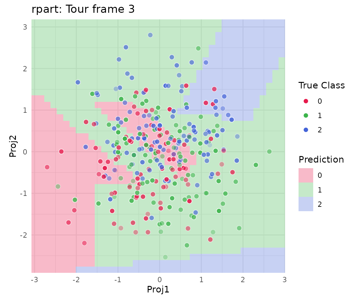
Step 4: Visualize at one tour frame

Each element of tour_history is a p × 2 orthonormal basis matrix. Extract a frame, construct the projection list, compute the boundary for each model, and plot.

if (requireNamespace("tourr", quietly = TRUE) && exists("tour_history")) {
  # Use frame 3 as an example
  frame_idx <- 3
  basis <- matrix(tour_history[, , frame_idx], nrow = length(feat_cols), ncol = 2)
  rownames(basis) <- feat_cols

  proj_list <- list(basis = basis, center = center_vals, scale = scale_vals)

  # Forward-project the training data to get axis ranges
  x_mat <- scale(d[, feat_cols], center = center_vals, scale = scale_vals)
  z_mat <- x_mat %*% basis
  ranges <- list(
    Proj1 = range(z_mat[, 1]) + c(-0.3, 0.3),
    Proj2 = range(z_mat[, 2]) + c(-0.3, 0.3)
  )
  colnames(basis) <- c("Proj1", "Proj2")
  proj_list$basis <- basis

  # Compute boundary for rpart at this frame
  b_rpart <- boundary_compute(m_rpart,
    feature_range = ranges, resolution = 40,
    projection = proj_list
  )
  plot_boundary(b_rpart,
    obs_data = d, true_label = "Y",
    x_col = "Proj1", y_col = "Proj2"
  ) +
    ggplot2::ggtitle("rpart: Tour frame 3")
}

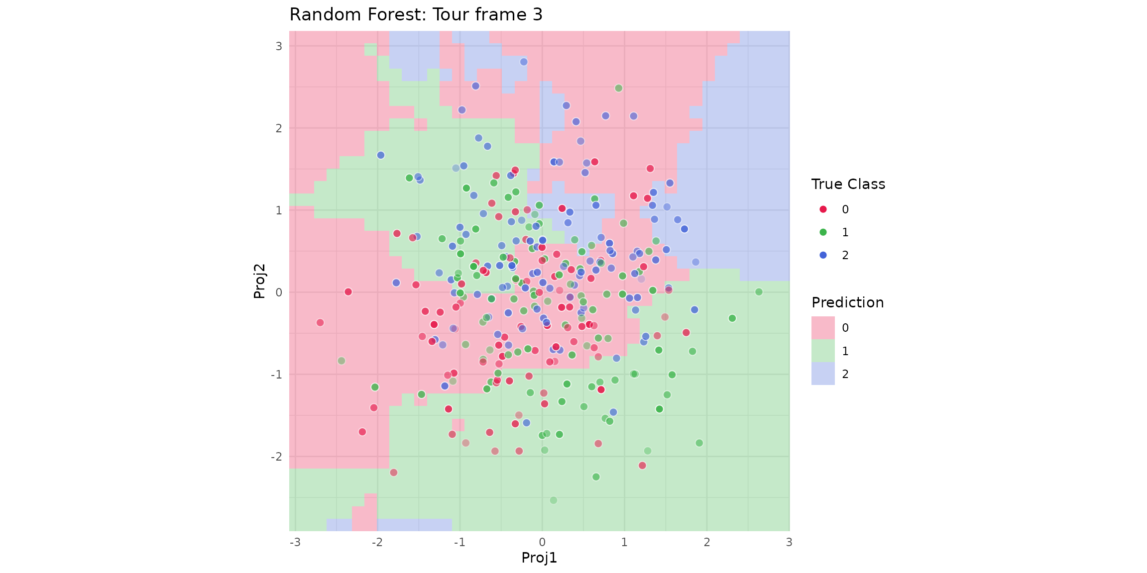
Step 5: Compare models at the same frame

Because both models are visualized using the same projection, the regions are directly comparable.

if (requireNamespace("tourr", quietly = TRUE) && exists("tour_history")) {
  b_rf <- boundary_compute(m_rf,
    feature_range = ranges, resolution = 40,
    projection = proj_list
  )
  plot_boundary(b_rf,
    obs_data = d, true_label = "Y",
    x_col = "Proj1", y_col = "Proj2"
  ) +
    ggplot2::ggtitle("Random Forest: Tour frame 3")
}

Animating the tour (optional)

To create an animated tour, iterate over all frames and display each plot in sequence. In an interactive R session you can use tourr::animate() directly with custom display functions, or save individual frames and combine them with the animation or gganimate packages.

# Pseudocode (adapt based on your animation workflow)
for (i in seq_len(dim(tour_history)[3])) {
  basis_i <- matrix(tour_history[, , i], nrow = length(feat_cols), ncol = 2)
  rownames(basis_i) <- feat_cols
  colnames(basis_i) <- c("Proj1", "Proj2")
  proj_i <- list(basis = basis_i, center = center_vals, scale = scale_vals)

  b <- boundary_compute(m_rpart,
    feature_range = ranges, resolution = 40,
    projection = proj_i
  )
  p <- plot_boundary(b,
    obs_data = d, true_label = "Y",
    x_col = "Proj1", y_col = "Proj2"
  )
  print(p)
}

Key points

• Generate one tour path; reuse it for every model.
• All models must be trained on the same set of numeric features.
• Use rownames(basis) <- feat_cols and colnames(basis) <- c("Proj1", "Proj2") to match the feature order expected by boundary_compute().
• The center and scale vectors reverse any standardization applied before touring, ensuring the boundary grid is mapped back to the correct feature space.